Gradient descent for multiple variables

Continue from the preceding example

[Ex]
\begin{array}{llll}
\hfill\mathrm{Size~in~feet^2 (x_1)}\hfill &
\hfill\mathrm{\#~bedrooms(x_2)}\hfill &
\hfill\mathrm{\#~ floors(x_3)}\hfill &
\hfill\mathrm{Age(x_4)}\hfill &
\hfill\mathrm{Price~$1000~(y)}\hfill

\\ \hline
\\ 2104 & 5 & 1 & 45& 460
\\ 1416 & 3&2&40&232
\\ 1534 & 3&2&30&315
\\ 852 & 2&1&36&178
\\ ... & ...& ...& ...& ...
\\ \end{array}

Notation:

• n = number of variables
• m = number of examples
• \(x^{(i)}\) = input variables of  \(i^{th}\) training example.
• \(x^{(i)}_j\) = value of input variable j  in \(i^{th}\) training example.

Hypothesis: \( h_\theta(x) = \theta_0 + \theta_1 x_1 + \theta_2 x_2 + \theta_3 x_3 + \theta_4 x_4\)

For convenience of notation, define \(x_0 = 1\), it means \( x^{(i)}_0 = 1\), so the hypothesis can transfer as:

$h_\theta(x) = \theta_0 x_0 + \theta_1 x_1 + \theta_2 x_2 + \theta_3 x_3 + \theta_4 x_4 $

         $       = \theta^T x $

So, the definition is as below:

[Def]
$$\begin{align*}& \text{repeat until convergence:} \; \lbrace \newline \; & \theta_j := \theta_j - \alpha \frac{1}{m} \sum\limits_{i=1}^{m} (h_\theta(x^{(i)}) - y^{(i)}) \cdot x_j^{(i)} \; & \text{for j := 0...n}\newline \rbrace\end{align*}$$

Batch gradient descent

[Ex]
Continue from the preceding article about cost function, here we will use this method to minimize the cost function, and using just two parameters \( \theta_0 \) and  \(\theta_1\) . It's a more general algorithm, and not only in linear regression.

outline:

• start with some  \( \theta_0 \) and  \(\theta_1\) 
• keep changing the  \( \theta_0 \) and  \(\theta_1\)  to reduce the \( J(\theta_0, \theta_1)\) and end up at a minimum

[Def]
repeat until converge {
\( \theta_j := \theta_j - \alpha \frac{\partial}{\partial \theta_j} J(\theta_0, \theta_1)  \)        (for j = 0 and j = 1)
}

\( \alpha\) : learning rate, it means how big step we take with creating descent.
Each step of gradient descent uses ALL the training examples.

Notice: we need updating these parameters "simultaneously" !

[Ex]
Back to our example, we take one parameter \( \theta_1\) now to get this algorithm more simpler.
[Plot 1]

Assuming this is our cost function, and if our  \( \theta_1\) starting from the blue point, since the slope is positive, so the new \( \theta_1\) from the gradient descent will decrease and  move to the green point (minimum), the moving speed depend on the \(\alpha\). In contrast, if our  \( \theta_1\) starting from the red point, it'll increase and move to the green point, too.

Although the moving speed is depend on the \(\alpha\), when \(\alpha\) is bigger the converging speed is more faster, but if the \(\alpha\) is too big, the result will be diverging.
[Plot 2]

On the contrary, if the \(\alpha\) is too small, it'll take too much time to converge.
[Plot 3]

Here is the other property of gradient descent, if our initial  \( \theta_1\) is at the local optimum, then it leaves \( \theta_1\) unchanged, because the slope will nearly equal to zero.
[Plot 4]

So, as we approach a local minimum, the gradient descent will automatically take smaller steps, this is why we don't need to decrease \(\alpha\) over time.

[For linear regression]
[Def]
$$\frac{\partial}{\partial \theta_j}J(\theta_0,\theta_1) = \frac{\partial}{\partial \theta_j}\frac{1}{2m} \sum_{i=1}^{m}(h_\theta(x^{(i)})-y^{(i)})^2$$

\( \begin{align*} \text{repeat until convergence: } \lbrace & \newline \theta_0 := & \theta_0 - \alpha \frac{1}{m} \sum\limits_{i=1}^{m}(h_\theta(x_{i}) - y_{i}) \newline \theta_1 := & \theta_1 - \alpha \frac{1}{m} \sum\limits_{i=1}^{m}\left((h_\theta(x_{i}) - y_{i}) x_{i}\right) \newline \rbrace& \end{align*}\)

Cost Function

[Ex]
Here is our training set and hypothesis as below:
\begin{array}{ll}
\hfill\mathrm{Size~in~feet^2 (x)}\hfill & \hfill\mathrm{Price($)~in~1000's(y)}\hfill
\\ \hline
\\ 2104 & 460
\\ 1416 & 232
\\ 1534 & 315
\\ 852 & 178
\\ ... & ...
\\ \end{array}

In this example, we want to fit a straight line to predict the house price, then we set a simple model.
Hypothesis: \( h_\theta(x) = \theta_0 + \theta_1 x\)

It's a simple regression problem, you can choose any number for \( \theta_0\) and \( \theta_1\), so that we can get the \( h_\theta(x)\) and it's meaning the value which the model predict to the input x. As a prediction model, we want the difference between \( h_\theta(x) \) and y to be small, in other words
is this hypothesis good fit to the data?

We can measure the accuracy of our hypothesis function by using a cost function or called squared error function, in other words it's almost the same as MSE in statistics.

[Def]
$$J(\theta_0, \theta_1) = \dfrac {1}{2m} \displaystyle \sum _{i=1}^m \left ( \hat{y}_{i}- y_{i} \right)^2 = \dfrac {1}{2m} \displaystyle \sum _{i=1}^m \left (h_\theta (x_{i}) - y_{i} \right)^2$$
m: the number of training example
\( h_\theta(x) \): form of hypothesis

Introduction

Machine Learning

Def 1 : 

The field of study that gives computers the ability to learn without being explicitly programmed.     --Arthur Samuel

Def 2 :

 A computer program is said to learn from experience E with respect to some class  of tasks T and performance measured P, if its performance at tasks in T, as measured by P, improve with experience E.     --Tom Mitchell

Any ML problems can assigned to one of two broad classifications:

• Supervised learning

    We are given a data set and already know what our correct output should look like, having the idea that there is a relationship between the input and the output.  
 
In a regression problem, we are trying to predict results within a continuous output.
In a classification problem, we are instead trying to predict results in a discrete output.

Example :

   
     Regression - 
    Given a picture of a person, we have to predict their age on the basis of the given picture

    Classification - 

    Given a patient with a tumor, we have to predict whether the tumor is malignant or benign.

• Unsupervised learning

    Unsupervised learning allows us to approach problems with little or no idea what our results should look like. We can derive structure from data where we don't necessarily know the effect of the variables.

Example :

    

    Clustering-

    Take a collection of 1,000 different genes, and find a way to group these genes into groups that are similar or related by different variables.

    Non-Clustering-

    The "Cocktail Party Algorithm", this algorithm can identify individual voices and music from a mesh of sounds at a cocktail party.

At last, all the article is the course's note from the "coursera", when it added the label [Machine Learning teached by Andrew Ng] 

Fuzzy Logic brief introduction

Fuzzy Logic

In the traditional computer logic, the truth value could be 0 or 1, so if we ask a question to computer :

" Is it cold today? " the answer will only "Yes" or "No". It cannot understand " a little cold" or " very

cold ", but Fuzzy logic can handle the concept of truth with many value between completely true and

completely false, it helps AI to take an important step.

As the below plot, the temperature is separated by dichotomy logic, cold or not called crisp set.

 But human's feeling often contain ambiguous narratives in semantics, in order to express more

accurately, the dichotomy extend to many-valued logic.

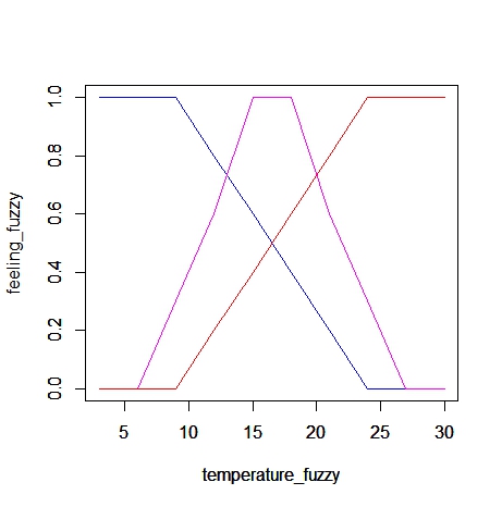
An fuzzy set called "membership function", it is a set of numbers which mapping between truth and

psychological. For example,  the following are 4 commonly used membership functions:

We can understand the relationship easily between the temperature and the degree of each word.

Fuzzy Inference

rules:

IF ___ IS ___ , THEN ___ IS ___ .

ex:

IF _temperature_ IS _ cold_ , THEN _fan speed_ IS _slow_ .

IF _temperature_ IS _ hot_ , THEN _fan speed_ IS _high_ .

Zadeh operators

NOT x = (1 - truth(x))

x AND y = minimum(truth(x), truth(y))

x OR y = maximum(truth(x), truth(y))

Fuzzy Logic vs Probability

Fuzzy logic is using pretty much the same tools as probability theory. But it's using them to trying to

capture a very different idea. Fuzzy logic is all about degrees of truth - about fuzziness and partial or

relative truths. Probability theory is interested in trying to make predictions about events from a state

of partial knowledge. But probability theory says nothing about how to reason about things that aren't

entirely true or false.