Overfitting

Continuing the preceding example of house price
Here is our training data as below plot
[Plot 1]

If we fit a linear function $\theta_0 + \theta_1 x$ to this data as below plot
[Plot 2]

It roughly means it's not fitting the training data very well, having very strong preconception. In this situation we called under fit and high bias.

If we use a quadratic function $\theta_0 + \theta_1 x + \theta_2 x^2$, then this function fit this data well.

[Plot 3]

And if we fit a fourth polynomial $\theta_0 + \theta_1 x + \theta_2 x^2 + \theta_3 x^3 + \theta_4 x^4$ to the data, then it's maybe look like this plot

[Plot 4]

Although, it fit the data very well, but it's not make any sense about the relationship between house price and size, this problem we called overfitting and high variance. We don't have enough data to constrain it to give us a good hypothesis.

Overfitting:

If we have too many features, the learned hypothesis may fit the training data very well, but fail to generalize to new examples.

Options:

• Reduce number of features
• manually select
• model selection algorithm

By throwing away some of features, it throw away some information at the same time.

• Regularization ,link: regularization
• Keep all the features, but reduce the magnitude / value of parameters
• Each will contribution a bit to predict y

Regularization

Continuing the preceding example

In our high-order polynomial function, it's the same as quadratic function except the $\theta_3$ and $\theta_4$ terms. Our goal is to minimize this function $\dfrac {1}{2m} \displaystyle \sum _{i=1}^m \left (h_\theta (x_{i}) - y_{i} \right)^2$, so if we decrease the influence from $\theta_3$ and $\theta_4$ in the cost function, just add some large number multiply the parameters,
$\dfrac {1}{2m} \displaystyle \sum _{i=1}^m \left (h_\theta (x_{i}) - y_{i} \right)^2 + 10000 \theta_3 + 10000 \theta_4$
then these parameters will become very close to 0, we make this high-order polynomial function approach to the fitted well quadratic function and less prone to overfit.


[In linear regression]

[Def ]
$$min_\theta\ \dfrac{1}{2m}\ \left[ \sum_{i=1}^m (h_\theta(x^{(i)}) - y^{(i)})^2 + \lambda\ \sum_{j=1}^n \theta_j^2 \right]$$

$\lambda$ is the regularization parameter, it decide how much these parameters are inflated.

[Gradient descent with regularization]
\begin{align*} & \text{Repeat}\ \lbrace \newline & \ \ \ \ \theta_0 := \theta_0 - \alpha\ \frac{1}{m}\ \sum_{i=1}^m (h_\theta(x^{(i)}) - y^{(i)})x_0^{(i)} \newline & \ \ \ \ \theta_j := \theta_j - \alpha\ \left[ \left( \frac{1}{m}\ \sum_{i=1}^m (h_\theta(x^{(i)}) - y^{(i)})x_j^{(i)} \right) + \frac{\lambda}{m}\theta_j \right] &\ \ \ \ \ \ \ \ \ \ j \in \lbrace 1,2...n\rbrace\newline & \rbrace \end{align*}

We separate this formula to get more intuition on this equation.
$$\theta_j := \theta_j(1 - \alpha\frac{\lambda}{m}) - \alpha\frac{1}{m}\sum_{i=1}^m(h_\theta(x^{(i)}) - y^{(i)})x_j^{(i)}$$

This equation can separate by two part, $\alpha\frac{1}{m}$ is greater then 0 in the first part, it means it''ll decrease $\theta$ a little bit, and the second part is the same with non-regularization.

[Normal equation with regularization]
\begin{align*}& \theta = \left( X^TX + \lambda \cdot L \right)^{-1} X^Ty \newline& \text{where}\ \ L = \begin{bmatrix} 0 & & & & \newline & 1 & & & \newline & & 1 & & \newline & & & \ddots & \newline & & & & 1 \newline\end{bmatrix}\end{align*}

It need notice that the matrix whose upper left entry is zero, since the intercept doesn't need regularization.The other advantage is in the m < n case, this normal equation in linear regression with regularization will be invertible, we have mentioned on this post normal-equation before, it is non-invertible or sigular when not added the regularization term in the m < n case.


[In logistic regression]

[Def]
$$J(\theta) = - \frac{1}{m} \sum_{i=1}^m \large[ y^{(i)}\ \log (h_\theta (x^{(i)})) + (1 - y^{(i)})\ \log (1 - h_\theta(x^{(i)}))\large] + \frac{\lambda}{2m}\sum_{j=1}^n \theta_j^2$$

[Gradient descent with regularization]
The gradient descent form is the same with linear regression, but the hypothesis is different.

Multi classification - one v.s all

[Ex]
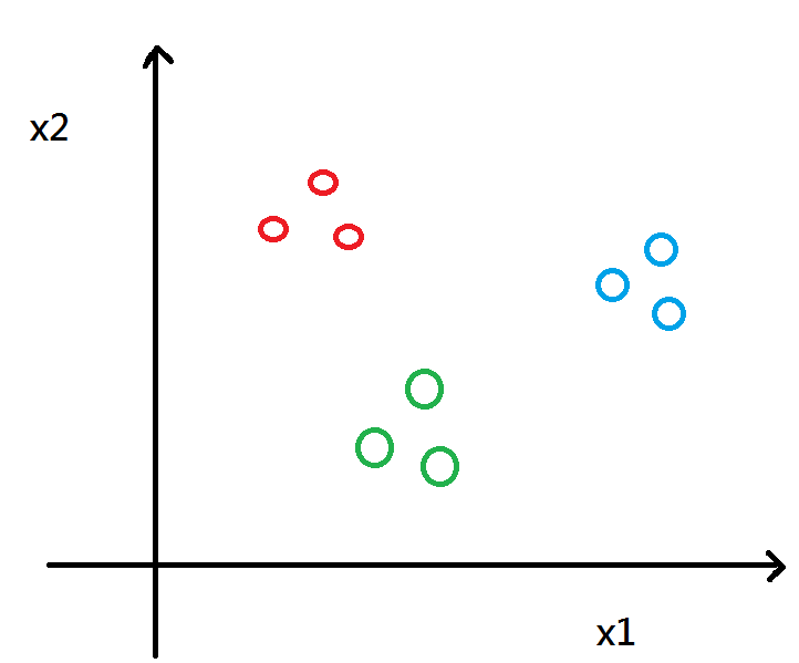
When the training data looks like this plot
[Plot 1]

We can use one v.s all classification help us.
First, we let red circle be the positive and the circle fill in purple as negative, then we may have the boundary $h_{\theta}^{(1)}(x)$ like this.
[Plot 2]

Second we let the green circle be the positive and the circle fill in purple as negative, then we can have the boundary $h_{\theta}^{(2)}(x)$ like this.
[Plot 3]

In the final, do the same thing, we can get the last boundary  $h_{\theta}^{(3)}(x)$ like this.
[Plot 4]

Concretely, we fit a classifier  $h_{\theta}^{(i)}(x)$ and estimate what is the probability that y = i class, or $ P(y = i | x ; \theta)$

So, to wrap up, if we want to classify an k-class problem, we need to train k classifier to solve the problem.

Logistic regression model

[Cost function in logistic regression]

[Def]
\begin{align*}& J(\theta) = \dfrac{1}{m} \sum_{i=1}^m \mathrm{Cost}(h_\theta(x^{(i)}),y^{(i)}) \newline & \mathrm{Cost}(h_\theta(x),y) = -\log(h_\theta(x)) \; & \text{if y = 1} \newline & \mathrm{Cost}(h_\theta(x),y) = -\log(1-h_\theta(x)) \; & \text{if y = 0}\end{align*}

Let's see the plot to get more clearly, first plot is y = 1
[Plot 1]

$h_{\theta}(x) = 1$ when y = 1, then the cost J = 0, but if $h_{\theta}(x) = 0$ then the cost $\rightarrow \infty$, for a further explanation,  if $h_{\theta}(x) = 0$ or $P( y = 1 | x, \theta) = 0$, but y = 1, we'll penalize the learning algorithm by a very large cost.

When y = 0, the plot is as below
[Plot 2]

Similarly, $-log(1 - h_\theta(x))$ will penalize the learning algorithm, if the result is opposite to the actual.

It's useful to use log here, let's take a look on this plot
[Plot 3]

It will stuck at local minimum when using square function in linear regression since it's non-convex, but when transfer by log in logistic regression, it'll guarantee to find the global minimum it's convex.

To combine this two case in one formula, we can get this equation:
[Def]
$$\mathrm{Cost}(h_\theta(x),y) = - y \; \log(h_\theta(x)) - (1 - y) \log(1 - h_\theta(x))$$
and the whole cost function is
$$J(\theta) = - \frac{1}{m} \displaystyle \sum_{i=1}^m [y^{(i)}\log (h_\theta (x^{(i)})) + (1 - y^{(i)})\log (1 - h_\theta(x^{(i)}))]$$

The next step is try to find the minimum of the cost function J with gradient descent which we had introduced before gradient-descent-for-multiple-variables, notice that it's needed updating simultaneously.

Classification - Binary

[Foreword]

[Ex]
Email: spam / not spam
Online transaction: fraudulent
Tumor: Malignant / Benign

y $\in$ {0, 1}

0: negative class ex: not spam, Benign tumor
1: positive class ex: spam, Malignant tumor

[Linear regression is not good]
Assume this is the hypothesis: $h_{\theta}(x) = \theta^T x$
then we set 0.5 as the threshold, that means

$h_{\theta}(x) \geq 0.5$, predict y = 1
$h_{\theta}(x) < 0.5$, predict y = 0

Here is the schematic diagram
[Plot 1]

When our data obtains the red point only, this threshold works well.
But when adding a purple point around there, the fitted line will get more flatten than before and it's not a good prediction.
Another funny thing is when we using linear regression for a classication problem, the hypothesis may output a value that are much larger or less than 1 and 0, even if the training example y only have 0 and 1.
So, this is the reason we will use another method which is called : Logistic regression.

[Logistic regression]
Because we want $0 \leq h_{\theta}(x) \leq 1$, so we using a function g to change the original  $h_{\theta}(x)$

$$\mathbf{h_{\theta}(x) = g(\theta^T x) = \frac{1}{1 + e^{-\theta^T x}}}$$

This formula is called "sigmoid function" or "logistic function"
We can use 0.5 as the threshold again through the sigmoid function, Let's take a loot on this plot
[Plot 2]

When $h_{\theta}(x) \geq 0.5$ means $ z \geq 0$, it'll output y = 1, in contrast $h_{\theta}(x) < 0.5 $ means $ z < 0, y = 0$


[Ex 1]
$h_{\theta}(x) = p( y = 1 | x , \theta) = $ estimate the probability that y = 1 on input x. So, if we input A patient's tumor size into the sigmoid function and get
$h_{\theta}(x) = 0.7 $
Then we can tell A there is 70% chance that this tumor being malignant.

[Ex 2]
Assume our data is below this plot and our $h_{\theta}(x) = \theta_0 + \theta_1 x_1 + \theta_2 x_2 + \theta_3 x_1^2 + \theta_4 x_2^2$,
[Plot 3]

we can get a divide circle when choose the fitted $\theta$ by Logistic regression as below plot.
$\theta = \lbrack  -1, 0, 0, 1, 1 \rbrack ^T$
It means this function will predict y = 1 when  $ -1 + x_1^2 + x_2^2 \geq 1$
[Plot 4]

This green circle is called decision boundary, the blue x means y = 1 and red o means y = 0