Batch gradient descent

[Ex]
Continue from the preceding article about cost function, here we will use this method to minimize the cost function, and using just two parameters \( \theta_0 \) and  \(\theta_1\) . It's a more general algorithm, and not only in linear regression.

outline:

• start with some  \( \theta_0 \) and  \(\theta_1\) 
• keep changing the  \( \theta_0 \) and  \(\theta_1\)  to reduce the \( J(\theta_0, \theta_1)\) and end up at a minimum

[Def]
repeat until converge {
\( \theta_j := \theta_j - \alpha \frac{\partial}{\partial \theta_j} J(\theta_0, \theta_1)  \)        (for j = 0 and j = 1)
}

\( \alpha\) : learning rate, it means how big step we take with creating descent.
Each step of gradient descent uses ALL the training examples.

Notice: we need updating these parameters "simultaneously" !

[Ex]
Back to our example, we take one parameter \( \theta_1\) now to get this algorithm more simpler.
[Plot 1]

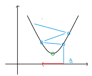
Assuming this is our cost function, and if our  \( \theta_1\) starting from the blue point, since the slope is positive, so the new \( \theta_1\) from the gradient descent will decrease and  move to the green point (minimum), the moving speed depend on the \(\alpha\). In contrast, if our  \( \theta_1\) starting from the red point, it'll increase and move to the green point, too.

Although the moving speed is depend on the \(\alpha\), when \(\alpha\) is bigger the converging speed is more faster, but if the \(\alpha\) is too big, the result will be diverging.
[Plot 2]

On the contrary, if the \(\alpha\) is too small, it'll take too much time to converge.
[Plot 3]

Here is the other property of gradient descent, if our initial  \( \theta_1\) is at the local optimum, then it leaves \( \theta_1\) unchanged, because the slope will nearly equal to zero.
[Plot 4]

So, as we approach a local minimum, the gradient descent will automatically take smaller steps, this is why we don't need to decrease \(\alpha\) over time.

[For linear regression]
[Def]
$$\frac{\partial}{\partial \theta_j}J(\theta_0,\theta_1) = \frac{\partial}{\partial \theta_j}\frac{1}{2m} \sum_{i=1}^{m}(h_\theta(x^{(i)})-y^{(i)})^2$$

\( \begin{align*} \text{repeat until convergence: } \lbrace & \newline \theta_0 := & \theta_0 - \alpha \frac{1}{m} \sum\limits_{i=1}^{m}(h_\theta(x_{i}) - y_{i}) \newline \theta_1 := & \theta_1 - \alpha \frac{1}{m} \sum\limits_{i=1}^{m}\left((h_\theta(x_{i}) - y_{i}) x_{i}\right) \newline \rbrace& \end{align*}\)